Plot retained activity
Create a spike raster and membrane-voltage figure from actual simulation outputs.
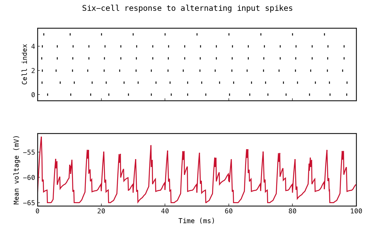
Simulate six COBA-LIF cells driven by alternating spikes on two input channels. Convert the actual output tensors into a validated Recording, then use FigureGrid to place a spike raster above a mean-voltage trace. The example saves both the figure and its retained numerical evidence.
Download the standalone script · View source
Run it
After installation, run from the repository root:
uv run python examples/plot_recording.pyFor the download, save the Python file and run it in an environment with snnlab installed. Every example is self-contained, uses CPU, and runs without a dataset download, Graphviz or FFmpeg.
Files, when produced, are written below artifacts/examples/plot_recording/ relative to your working directory. A repeated run replaces that example’s outputs.
Complete code
"""Simulate six cells and export a figure from their actual retained signals."""

from pathlib import Path

import matplotlib

matplotlib.use("Agg")
import matplotlib.pyplot as plt
import numpy as np
import torch

from snnlab import lang as snn
from snnlab import viz
from snnlab.sim.execution import ExecutionSpec, simulate


def main(out=Path("artifacts/examples/plot_recording")):
    net = snn.Network("raster_example", dt=0.1 * snn.ms)
    events = net.input(
        "events", shape=("time", "batch", 2), signal_type="spikes", unit="spike"
    )
    cells = net.population("cells", size=6, neuron=snn.COBA_LIF(tau_mem=20 * snn.ms))
    net.connect(
        events,
        cells.excitatory,
        name="drive",
        synapse=snn.AMPA(tau=2 * snn.ms),
        weight=snn.LowerClampedNormal(0.5, 0.1),
        constraint=snn.NonNegative(),
        connection="feedforward",
    )
    net.output("spikes", cells.spikes)
    net.output("voltage", cells.voltage)
    inputs = torch.zeros(1000, 1, 2)
    inputs[::100, 0, 0] = 1
    inputs[50::100, 0, 1] = 1
    result = simulate(
        ExecutionSpec(
            kind="simulate",
            executor="graph",
            graph=snn.compile(net).graph,
            inputs={"events": inputs},
            seed=17,
            device="cpu",
        )
    )
    recording = viz.Recording(
        dt_ms=0.1,
        signals={
            name: tensor.detach().numpy()[:, 0, :]
            for name, tensor in result.outputs.items()
        },
        metadata={"seed": 17, "description": "Illustrative six-cell simulation"},
    )
    spikes, voltage = recording.require("spikes", "voltage")
    time_ms = np.arange(recording.steps) * recording.dt_ms
    grid = viz.FigureGrid(
        rows=(1, 1), columns=1, bounds=(0.10, 0.12, 0.85, 0.76), row_gap=0.14
    )
    grid.place("raster", row=0, column=0)
    grid.place("voltage", row=1, column=0)
    figure = grid.figure(figsize=(8, 5))
    raster = figure.add_axes(grid.rect("raster").mpl)
    trace = figure.add_axes(grid.rect("voltage").mpl)
    steps, units = np.nonzero(spikes)
    raster.scatter(
        steps * recording.dt_ms, units, s=12, marker="|", color=grid.theme.ink
    )
    raster.set(xlim=(0, recording.duration_ms), ylim=(-0.5, 5.5), ylabel="Cell index")
    raster.tick_params(labelbottom=False)
    trace.plot(time_ms, voltage.mean(axis=1), color=grid.theme.accent)
    trace.set(
        xlim=(0, recording.duration_ms), xlabel="Time (ms)", ylabel="Mean voltage (mV)"
    )
    figure.suptitle("Six-cell response to alternating input spikes", fontsize=12)
    Path(out).mkdir(parents=True, exist_ok=True)
    figure.savefig(Path(out) / "recording.png", dpi=160)
    np.savez(Path(out) / "recording.npz", dt_ms=recording.dt_ms, **recording.signals)
    plt.close(figure)
    print(f"Recording: {recording.steps} steps, {recording.duration_ms:.1f} ms")
    print("Exported recording.png and recording.npz")


if __name__ == "__main__":
    main()
What to notice
- Output tensors include a batch axis. This example has one presentation and explicitly selects it before constructing the Recording.
Recording.require()fails if a requested signal is absent. The plotting code consumes the stored arrays rather than rerunning the simulation or filling missing signals.- Raster positions use source steps multiplied by the 0.1 ms timestep. The trace averages voltage across the six cells, not across repeated trials.
- FigureGrid uses named regions with normalized figure coordinates. Matplotlib's Agg backend exports a PNG without an interactive display.
The output directory contains recording.png and recording.npz, with dt_ms, spikes and voltage in the archive. Input channels spike every 10 ms, offset by 5 ms. The preview below was generated by this script with seed 17; it is one illustrative simulation, not an aggregate or uncertainty estimate.
Expected result
Recording: 1000 steps, 100.0 ms
Exported recording.png and recording.npz